Linear Mixed Models: Pulp Brightness and PSID Longitudinal Data

Faraway (2016) Sections 10.1 and 11.1

Published

April 15, 2026

Faraway (2016) Section 10.1: Pulp Brightness

Data Loading

This script demonstrates linear mixed effects models using the lme4 package, by Bates et al. (2015), using the example in Faraway (2016) section 10.1, page 200. This package is the standard package for fitting mixed effects models.

The first dataset we use measures paper brightness (continuous response) depending on which shift operator prepared the pulp.

Code

library(conflicted)
library(dplyr)
library(faraway)
library(ggplot2)
library(lme4)

Loading required package: Matrix

As always we can run ?pulp to get information about the dataset:

Code

?pulp

Code

pulp_tbl <- as_tibble(pulp)
pulp_tbl

# A tibble: 20 × 2
   bright operator
    <dbl> <fct>   
 1   59.8 a       
 2   60   a       
 3   60.8 a       
 4   60.8 a       
 5   59.8 a       
 6   59.8 b       
 7   60.2 b       
 8   60.4 b       
 9   59.9 b       
10   60   b       
11   60.7 c       
12   60.7 c       
13   60.5 c       
14   60.9 c       
15   60.3 c       
16   61   d       
17   60.8 d       
18   60.6 d       
19   60.5 d       
20   60.5 d

We can see that there are 20 observations of brightness, with 5 measurements for each of 4 operators.

We want to model brightness using an intercept only model with random operator effects.

SELF TEST: What is the mathematical formulation of this model?

The model is: \[ y_{ij} = \beta_0 + b_i + \varepsilon_{ij} \] where $y_{ij}$ is the brightness for the $j$-th measurement of the $i$-th operator, $\beta_0$ is the overall mean brightness (fixed effect), $b_i \sim N(0, \sigma_b^2)$ is the random effect for operator $i$, and $\varepsilon_{ij} \sim N(0, \sigma_{\varepsilon}^2)$ is the observation-level error.

We estimate $\beta_0$ as the fixed effect, and $\sigma_b^2$ and $\sigma_{\varepsilon}^2$ as the variance components for the random effects and residuals, respectively.

We fit a model using a REML criterion, and a model using a MLE criterion, to compare the results.

SELF TEST: REML vs. MLE in linear mixed models

In mixed effects models we need to estimate the variance components (random effects variance and residual variance) in addition to the fixed effects. The standard MLE estimate has a strong downward bias for variance components (it will underestimate them). REML corrects for this bias.

Code

m_pulp_reml <- lmer(bright ~ 1 + (1 | operator), pulp_tbl)
m_pulp_mle <- lmer(bright ~ 1 + (1 | operator), pulp_tbl, REML = FALSE)

lme4::lmer() Syntax

lme4::lmer() uses the pattern response ~ fixed effects + (random effects | group), data = .... The second argument is the data frame, and REML = FALSE switches from REML to MLE. Here (1 | operator) gives a random intercept for each operator.

Note that the 1 + in the fixed effects is optional since the intercept is included by default, but here it is included explicitly for clarity.

The m_pulp_reml object is of class lmerMod. Let’s examine both fits:

Code

sum_pulp_reml <- summary(m_pulp_reml)
sum_pulp_reml

Linear mixed model fit by REML ['lmerMod']
Formula: bright ~ 1 + (1 | operator)
   Data: pulp_tbl

REML criterion at convergence: 18.6

Scaled residuals: 
    Min      1Q  Median      3Q     Max 
-1.4666 -0.7595 -0.1244  0.6281  1.6012 

Random effects:
 Groups   Name        Variance Std.Dev.
 operator (Intercept) 0.06808  0.2609  
 Residual             0.10625  0.3260  
Number of obs: 20, groups:  operator, 4

Fixed effects:
            Estimate Std. Error t value
(Intercept)  60.4000     0.1494   404.2

We get one fixed effect (the overall mean brightness) and one random effect (the operator-level variation).

DENNIS TO ADD SOME EXPOSITION ON THE STANDARD ERROR OF FIXED EFFECTS HERE

For the random effect we get two variance parameters. The Residual variance is the estimated variance $\sigma_{\varepsilon}^2$ of the obervation-level errors $\varepsilon_{ij}$, while the operator variance is the estimated variance $\sigma_b^2$ of the operator-level random effects $b_i$. Here the value reported by Std.Dev. is just the square root of the variance (not a standard error of the variance estimate).

We can also see the estimates for the MLE fit:

Code

summary(m_pulp_mle)

Linear mixed model fit by maximum likelihood  ['lmerMod']
Formula: bright ~ 1 + (1 | operator)
   Data: pulp_tbl

      AIC       BIC    logLik -2*log(L)  df.resid 
     22.5      25.5      -8.3      16.5        17 

Scaled residuals: 
     Min       1Q   Median       3Q      Max 
-1.50554 -0.78116 -0.06353  0.65850  1.56232 

Random effects:
 Groups   Name        Variance Std.Dev.
 operator (Intercept) 0.04575  0.2139  
 Residual             0.10625  0.3260  
Number of obs: 20, groups:  operator, 4

Fixed effects:
            Estimate Std. Error t value
(Intercept)  60.4000     0.1294   466.7

We can see that (as expected) the MLE variance estimates are smaller than the REML estimates, while the fixed effect estimate is the same.

We can directly extract the fixed effect estimates:

Code

tibble(
  REML = fixef(m_pulp_reml),
  MLE = fixef(m_pulp_mle)
)

# A tibble: 1 × 2
   REML   MLE
  <dbl> <dbl>
1  60.4  60.4

Caution

The fixed effect estimates here are the same between REML and MLE, only because the design is balanced. Generally they will differ for unbalanced designs.

DENNIS: TO ADD MORE CONTEXT IF NEEDED, CLAIM IS THAT REML VARIANCE ESTIMATES MUST BE SCALAR MULTIPLE OF MLE VARIANCE ESTIMATES IN BALANCED DESIGNS

Extracting Model Components

Usually we don’t extract the random effects estimates directly (since there is only a posterior distribution), but we can extract the conditional modes using the generic method lme4::ranef():

Code

as_tibble(ranef(m_pulp_reml))

# A tibble: 4 × 5
  grpvar   term        grp   condval condsd
  <chr>    <fct>       <fct>   <dbl>  <dbl>
1 operator (Intercept) a      -0.122  0.127
2 operator (Intercept) b      -0.259  0.127
3 operator (Intercept) c       0.168  0.127
4 operator (Intercept) d       0.213  0.127

Since the conditional distribution is normal, the conditional modes are also the conditional means.

Variance-covariance matrix for the fixed effects:

Code

sum_pulp_reml$vcov

1 x 1 Matrix of class "dpoMatrix"
            (Intercept)
(Intercept)  0.02233333

This is a constant in this case since we are only estimating one fixed effect (the intercept).

We can directly access the estimated residual standard deviation $\sigma_{\varepsilon}$:

Code

sum_pulp_reml$sigma

[1] 0.3259601

We can access both variance-covariance components ($\sigma_b^2$ and $\sigma_{\varepsilon}^2$):

Code

sum_pulp_reml$varcor

 Groups   Name        Std.Dev.
 operator (Intercept) 0.26093 
 Residual             0.32596

And the usual generic method coef() function gives us the fixed effect coefficient table:

Code

coef(sum_pulp_reml)

            Estimate Std. Error  t value
(Intercept)     60.4  0.1494434 404.1664

Hand-Computed Fixed Effect Estimate

Since fixed effect estimates for linear mixed models are a special case of solving a generalised least squares (GLS) estimator, we can verify the fixed effect estimate by hand-computing the GLS solution from the estimated variance structure:

Code

components <- as_tibble(VarCorr(m_pulp_reml))$vcov
components

[1] 0.06808334 0.10625000

Code

Vi <- components[2] * diag(5) + components[1] * matrix(1, nrow = 5, ncol = 5)
V <- bdiag(Vi, Vi, Vi, Vi)
Z <- rep(1, 20)

What This Code Does and Syntax Notes

components <- tibble::as_tibble(lme4::VarCorr(m_pulp_reml))$vcov extracts estimated variance components from the fitted model. lme4::VarCorr(...) returns random-effect and residual variance information, tibble::as_tibble(...) turns it into a tidy table, and $vcov selects the variance column.
Vi <- components[2] * ... builds the $5 \times 5$ covariance matrix for one operator. diag(5) creates an identity matrix, and matrix(1, nrow = 5, ncol = 5) creates a $5 \times 5$ matrix of ones.
V <- Matrix::bdiag(Vi, Vi, Vi, Vi) creates a block-diagonal covariance matrix for all 4 operators. Matrix::bdiag(...) stacks the operator-level covariance blocks on the diagonal.
Z <- rep(1, 20) creates the intercept-only fixed-effect design vector for all 20 observations.

Hand-computed GLS estimate of the fixed effect (intercept):

Code

(1 / (t(Z) %*% solve(V) %*% Z)) * t(Z) %*% solve(V) %*% pulp$bright

1 x 1 Matrix of class "dgeMatrix"
     [,1]
[1,] 60.4

Hand-computed standard error (GLS covariance):

Code

sqrt(1 / (t(Z) %*% solve(V) %*% Z))

1 x 1 Matrix of class "dgeMatrix"
          [,1]
[1,] 0.1494434

Model Diagnostics

This course does not focus on model diagnostics, but the general idea behind these plots is to evaluate whether our model assumptions are met. The default residuals function accounts for the estimated random effects. These residuals can be regarded as estimates of the observation-level errors $\varepsilon_{ij}$, which is usually what we want for diagnostics:

Code

resid_m_pulp_reml <- residuals(m_pulp_reml)
fitted_m_pulp_reml <- fitted(m_pulp_reml)
diagnostics_tbl <- tibble(residual = resid_m_pulp_reml, fitted = fitted_m_pulp_reml)

ggplot(diagnostics_tbl, aes(sample = residual)) +
  stat_qq() +
  stat_qq_line() +
  labs(x = "Theoretical Quantiles", y = "Residuals") +
  theme_minimal()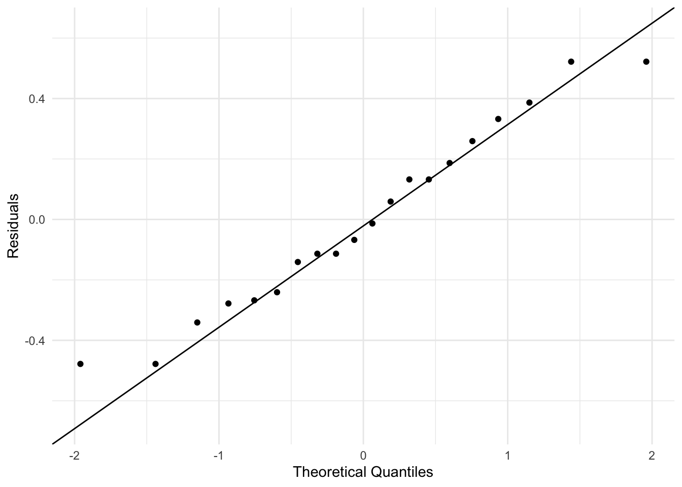

Code

ggplot(diagnostics_tbl, aes(x = fitted, y = residual)) +
  geom_point() +
  geom_hline(yintercept = 0, linewidth = 0.5) +
  labs(x = "Fitted", y = "Residuals") +
  theme_minimal()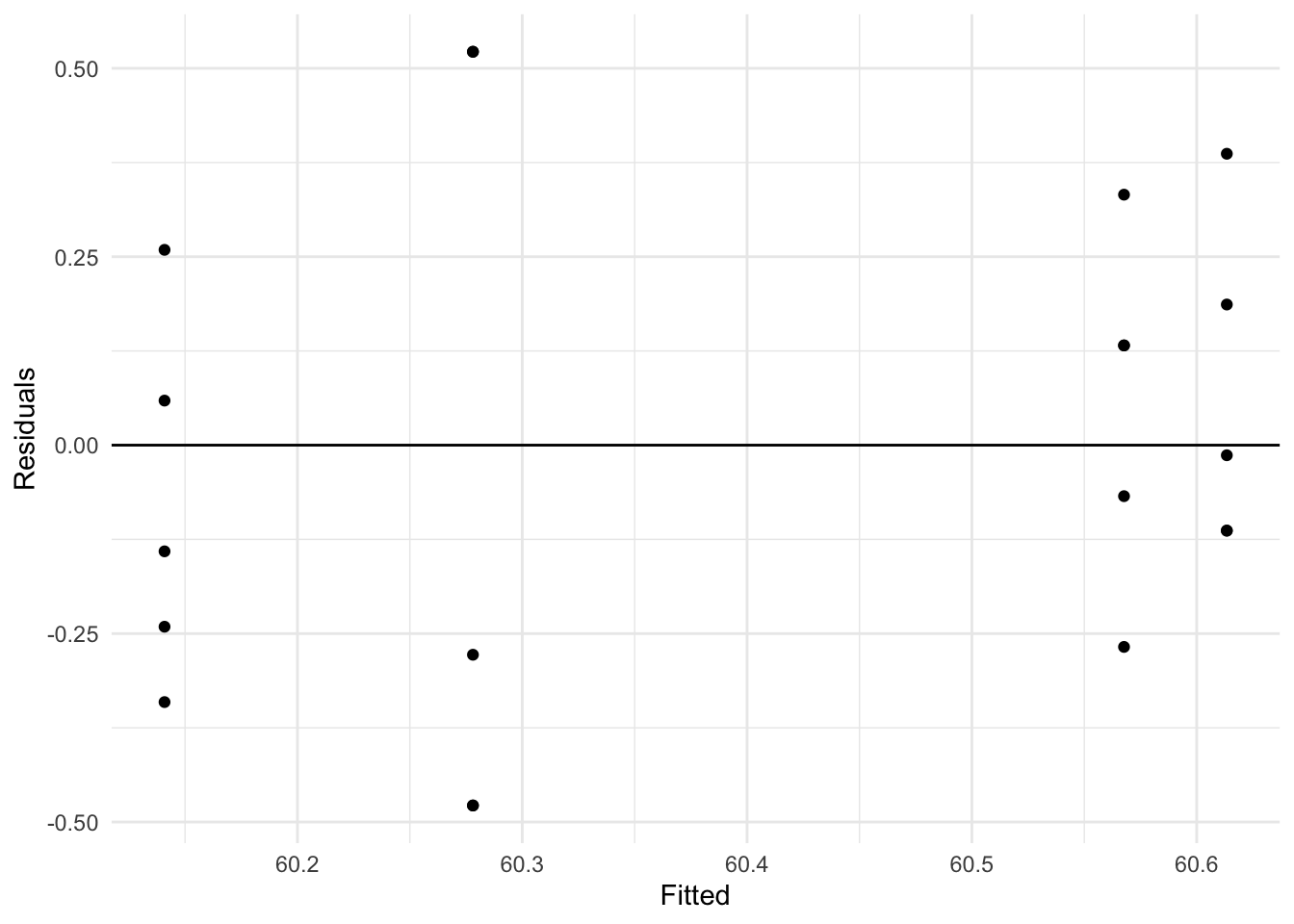

These plots show that it is a reasonable assumption that the residuals are approximately normally distributed and have constant variance across fitted values.

Note

We can compute residuals by hand to verify:

Code

operator_intercept <- ranef(m_pulp_reml)[["operator"]][["(Intercept)"]]
residual_manual <- pulp$bright - rep(operator_intercept, each = 5) - fixef(m_pulp_reml)[["(Intercept)"]]

Verify they match the model output:

Code

all(residual_manual == residuals(m_pulp_reml))

[1] TRUE

Faraway (2016) Section 11.1: PSID Longitudinal Data

Now we fit a model with random slopes. The Panel Study of Income Dynamics (PSID) dataset tracks income over time for individuals. We use log(income) as the response.

Load and examine data:

Code

?psid

So this dataset has 1,661 observations on the following 6 variables:

age: age in 1968
educ: years of education
sex: sex of individual (F or M)
income: annual income in dollars
year: calendar year
person: ID number for individual

Code

psid_tbl <- as_tibble(psid)
psid_tbl

# A tibble: 1,661 × 6
     age  educ sex   income  year person
   <int> <int> <fct>  <int> <int>  <int>
 1    31    12 M       6000    68      1
 2    31    12 M       5300    69      1
 3    31    12 M       5200    70      1
 4    31    12 M       6900    71      1
 5    31    12 M       7500    72      1
 6    31    12 M       8000    73      1
 7    31    12 M       8000    74      1
 8    31    12 M       9600    75      1
 9    31    12 M       9000    76      1
10    31    12 M       9000    77      1
# ℹ 1,651 more rows

We create a new variable cyear, the time relative to 1978

Code

psid_tbl <- mutate(psid_tbl, cyear = year - 78)

Note

Centering predictors: By centering year at 1978, the intercept in our model will represent log-income in 1978.

REML vs. MLE with Random Slopes

We fit models with both random intercept and random slope (person growth rate varies) using both the REML (default) and the biased MLE (REML = FALSE) estimation methods:

Code

m_psid_reml <- lmer(
  log(income) ~ cyear * sex + age + educ + (cyear | person),
  data = psid_tbl
)

m_psid_mle <- lmer(
  log(income) ~ cyear * sex + age + educ + (cyear | person),
  data = psid_tbl,
  REML = FALSE
)

Note

(cyear | person) gives both a random intercept and slope for each person.

SELF TEST: What is the mathematical formulation of this model?

The model is: \[ \begin{split} \log(\texttt{income})_{ij} &= \beta_0 + \beta_1 \texttt{cyear}_{j} + \beta_2 \mathbb{1}(\texttt{sex}_{i}=\texttt{M}) + \beta_3 \texttt{age}_{i} + \beta_4 \texttt{educ}_{i}\\ &\quad + \beta_5 \texttt{cyear}_{j}\mathbb{1}(\texttt{sex}_{i}=\texttt{M}) + b_{0i} + b_{1i}\texttt{cyear}_{j} + \varepsilon_{ij} \end{split} \] where $\log(\texttt{income}_{ij})$ corresponds to person $i$ at time $j$, and $\mathbb{1}(\texttt{sex}_{i}=\texttt{M})$ corresponds to the sexM coefficient in the output. The random effects are correlated: \[ \begin{pmatrix} b_{0i} \\ b_{1i} \end{pmatrix} \sim N\Biggl( \begin{pmatrix}0\\0\end{pmatrix}, \begin{pmatrix} \sigma_{b_0}^2 & \sigma_{b_{01}}\\ \sigma_{b_{01}} & \sigma_{b_1}^2 \end{pmatrix} \Biggr), \quad \varepsilon_{ij}\sim N(0,\sigma_\varepsilon^2). \]

Examine REML fit:

Code

s_psid_reml <- summary(m_psid_reml)
s_psid_reml

Linear mixed model fit by REML ['lmerMod']
Formula: log(income) ~ cyear * sex + age + educ + (cyear | person)
   Data: psid_tbl

REML criterion at convergence: 3819.8

Scaled residuals: 
     Min       1Q   Median       3Q      Max 
-10.2310  -0.2134   0.0795   0.4147   2.8254 

Random effects:
 Groups   Name        Variance Std.Dev. Corr
 person   (Intercept) 0.2817   0.53071      
          cyear       0.0024   0.04899  0.19
 Residual             0.4673   0.68357      
Number of obs: 1661, groups:  person, 85

Fixed effects:
             Estimate Std. Error t value
(Intercept)  6.674211   0.543323  12.284
cyear        0.085312   0.008999   9.480
sexM         1.150312   0.121292   9.484
age          0.010932   0.013524   0.808
educ         0.104209   0.021437   4.861
cyear:sexM  -0.026306   0.012238  -2.150

Correlation of Fixed Effects:
           (Intr) cyear  sexM   age    educ  
cyear       0.020                            
sexM       -0.104 -0.098                     
age        -0.874  0.002 -0.026              
educ       -0.597  0.000  0.008  0.167       
cyear:sexM -0.003 -0.735  0.156 -0.010 -0.011

The above summary is more complex than the previous example because we have more fixed effects and a more complex random effects structure. The Correlation of Fixed Effects table shows the correlation between the fixed effect estimates. The covariance matrix of the fixed effects estimates can easily be derived from this.

The Random effects table shows the variance components $\sigma_{b_0}^2$ and $\sigma_{b_1}^2$ for the random intercept and random slope $b_{1i}$, as well as their correlation (from which $\sigma_{b_{01}}$ can be calculated), and the residual variance $\sigma_\varepsilon^2$.

We can directly access the variance-covariance matrix of fixed effects:

Code

s_psid_reml$vcov

6 x 6 Matrix of class "dpoMatrix"
              (Intercept)         cyear          sexM           age
(Intercept)  2.952003e-01  9.887065e-05 -6.841728e-03 -6.419660e-03
cyear        9.887065e-05  8.099019e-05 -1.075138e-04  2.572365e-07
sexM        -6.841728e-03 -1.075138e-04  1.471185e-02 -4.311368e-05
age         -6.419660e-03  2.572365e-07 -4.311368e-05  1.828907e-04
educ        -6.954571e-03  2.976876e-08  2.136982e-05  4.831984e-05
cyear:sexM  -2.023534e-05 -8.099199e-05  2.313032e-04 -1.681985e-06
                     educ    cyear:sexM
(Intercept) -6.954571e-03 -2.023534e-05
cyear        2.976876e-08 -8.099199e-05
sexM         2.136982e-05  2.313032e-04
age          4.831984e-05 -1.681985e-06
educ         4.595265e-04 -2.838170e-06
cyear:sexM  -2.838170e-06  1.497587e-04

We can compare the fixed effect estimates from the REML and MLE fits:

Code

tibble(
  names = names(fixef(m_psid_reml)),
  REML = fixef(m_psid_reml),
  MLE = fixef(m_psid_mle)
)

# A tibble: 6 × 3
  names          REML     MLE
  <chr>         <dbl>   <dbl>
1 (Intercept)  6.67    6.68  
2 cyear        0.0853  0.0852
3 sexM         1.15    1.15  
4 age          0.0109  0.0109
5 educ         0.104   0.104 
6 cyear:sexM  -0.0263 -0.0262

Note that here the fixed effect estimates differ slightly between REML and MLE, which is to be expected.

Finally we can access at the standard errors of the fixed effects:

Code

sqrt(diag(s_psid_reml$vcov))

(Intercept)       cyear        sexM         age        educ  cyear:sexM 
0.543323402 0.008999455 0.121292411 0.013523710 0.021436569 0.012237594

As above, we can examine the variance-covariance of random effects:

Code

VarCorr(m_psid_reml)

 Groups   Name        Std.Dev. Corr 
 person   (Intercept) 0.530713      
          cyear       0.048988 0.187
 Residual             0.683574

Interpreting the Random Effects Output

The standard deviation of the random intercept tells us how much variability there is in initial log-income across individuals. Since income is on a log-scale, this values is multiplicative—95% of incomes are between $\exp(-2\sigma_{b_0})$= 0.35 and $\exp(2\sigma_{b_0})$= 2.89 times the overall mean income in 1978.

The standard deviation of the random slope tells us how much variability there is in income growth rates across individuals.

A low correlation value tells us that the slope of income growth over time, is minimally effected by the initial salary (intercept).

Package Citations and Session Information

Session Information

Code

sessionInfo()

R version 4.4.2 (2024-10-31)
Platform: x86_64-apple-darwin20
Running under: macOS Sequoia 15.7.5

Matrix products: default
BLAS:   /Library/Frameworks/R.framework/Versions/4.4-x86_64/Resources/lib/libRblas.0.dylib 
LAPACK: /Library/Frameworks/R.framework/Versions/4.4-x86_64/Resources/lib/libRlapack.dylib;  LAPACK version 3.12.0

locale:
[1] en_US.UTF-8/en_US.UTF-8/en_US.UTF-8/C/en_US.UTF-8/en_US.UTF-8

time zone: Australia/Melbourne
tzcode source: internal

attached base packages:
[1] stats     graphics  grDevices datasets  utils     methods   base     

other attached packages:
[1] lme4_1.1-38      Matrix_1.7-1     ggplot2_4.0.2    faraway_1.0.9   
[5] dplyr_1.2.0      conflicted_1.2.0

loaded via a namespace (and not attached):
 [1] gtable_0.3.6       jsonlite_2.0.0     compiler_4.4.2     renv_1.1.7        
 [5] tidyselect_1.2.1   Rcpp_1.1.1         scales_1.4.0       splines_4.4.2     
 [9] boot_1.3-31        yaml_2.3.12        fastmap_1.2.0      lattice_0.22-6    
[13] R6_2.6.1           labeling_0.4.3     generics_0.1.4     knitr_1.51        
[17] rbibutils_2.4.1    MASS_7.3-61        tibble_3.3.1       nloptr_2.2.1      
[21] minqa_1.2.8        RColorBrewer_1.1-3 pillar_1.11.1      rlang_1.1.7       
[25] utf8_1.2.6         cachem_1.1.0       xfun_0.56          S7_0.2.1          
[29] memoise_2.0.1      cli_3.6.5          withr_3.0.2        magrittr_2.0.4    
[33] Rdpack_2.6.5       digest_0.6.39      grid_4.4.2         rstudioapi_0.18.0 
[37] lifecycle_1.0.5    nlme_3.1-168       reformulas_0.4.4   vctrs_0.7.1       
[41] evaluate_1.0.5     glue_1.8.0         farver_2.1.2       rmarkdown_2.30    
[45] tools_4.4.2        pkgconfig_2.0.3    htmltools_0.5.9

Code

packages <- c("conflicted", "dplyr", "faraway", "ggplot2", "lme4")
for (pkg in packages) {
  cit <- citation(pkg)

  # Check if multiple citations
  if (length(cit) > 1) {
    cat("- **", pkg, "**:\n", sep = "")
    for (i in seq_along(cit)) {
      cit_text <- format(cit[i], style = "text")
      cat("    - ", cit_text, "\n\n", sep = "")
    }
  } else {
    cit_text <- format(cit, style = "text")
    cat("- **", pkg, "**: ", cit_text, "\n\n", sep = "")
  }
}

conflicted: Wickham H (2023). conflicted: An Alternative Conflict Resolution Strategy. R package version 1.2.0, https://github.com/r-lib/conflicted, https://conflicted.r-lib.org/.
dplyr: Wickham H, François R, Henry L, Müller K, Vaughan D (2026). dplyr: A Grammar of Data Manipulation. R package version 1.2.0, https://github.com/tidyverse/dplyr, https://dplyr.tidyverse.org.
faraway: Faraway J (2025). faraway: Datasets and Functions for Books by Julian Faraway. R package version 1.0.9, https://github.com/julianfaraway/faraway.
ggplot2: Wickham H (2016). ggplot2: Elegant Graphics for Data Analysis. Springer-Verlag New York. ISBN 978-3-319-24277-4, https://ggplot2.tidyverse.org.
lme4: Bates D, Mächler M, Bolker B, Walker S (2015). “Fitting Linear Mixed-Effects Models Using lme4.” Journal of Statistical Software, 67(1), 1-48. doi:10.18637/jss.v067.i01 https://doi.org/10.18637/jss.v067.i01.

References

Bates, Douglas, Martin Mächler, Ben Bolker, and Steve Walker. 2015. “Fitting Linear Mixed-Effects Models Using Lme4.” Journal of Statistical Software 67 (1): 1–48. https://doi.org/10.18637/jss.v067.i01.

Faraway, Julian J. 2016. Extending the Linear Model with r : Generalized Linear, Mixed Effects and Nonparametric Regression Models, Second Edition. Second edition. Chapman & Hall/CRC Texts in Statistical Science Series. Chapman; Hall/CRC. https://research.ebsco.com/plink/3806c0de-f79d-330d-9c4e-7bb136efaa53.