(Quasi-)Poisson GLM: Cell Differentiation Study

Fahrmeir and Tutz (2001) Examples 2.3, 2.6, and 2.7

Authors

Dennis Leung

Jacob Cumming

Published

March 12, 2026

Package Setup and Data

As in the previous script, for safety we import the conflicted package first to manage any function name conflicts.

Code

library(conflicted)

We import the other packages needed to complete the analysis.

Code

library(dplyr)
library(Fahrmeir)
library(gee)
library(geepack)
library(ggplot2)
library(MASS)

Thorough MASS documentation is available in the book Modern Applied Statistics with S (MASS) Venables and Ripley (2002) which is available to you for free.

Example 2.3 (p. 37): Cell Differentiation Data

Load and Inspect Data

We now attempt to replicate the results in Fahrmeir and Tutz (2001) Example 2.3 (p. 37). We import and preview the cells data from the Fahrmeir package. The purpose of this dataset is to explore whether the two agents stimulate cell differentiation synergistically (is an interaction between the agents) or independently.

Code

data(cells)
cells_tbl <- as_tibble(cells)
cells_tbl

# A tibble: 16 × 3
       y   TNF   IFN
   <int> <int> <int>
 1    11     0     0
 2    18     0     4
 3    20     0    20
 4    39     0   100
 5    22     1     0
 6    38     1     4
 7    52     1    20
 8    69     1   100
 9    31    10     0
10    68    10     4
11    69    10    20
12   128    10   100
13   102   100     0
14   171   100     4
15   180   100    20
16   193   100   100

All the variables are encoded as integers and so we do not need to manipulate the data types. It is also good practice in RStudio to run ?cells to inspect the documentation for the dataset.

Fit Poisson GLM Model

We initially just fit the Poisson GLM as in Ex 2.3.

What is the canonical link function for Poisson regression? Expand for answer.

The default link is the log link, meaning that we assume $\log(\texttt{y})$ depends linearly on the covariates.

Code

glm_poisson <- glm(formula = y ~ TNF * IFN, family = poisson, data = cells_tbl)

glm() Syntax Explanation

formula = y ~ TNF * IFN: Response variable y modeled with main effects and interaction for TNF and IFN. This is equivalent to y ~ 1 + TNF + IFN + TNF * IFN.
family = poisson: Specifies Poisson distribution with default log link function
data = cells_tbl: Data frame containing the variables

Inspect Results

We inspect the returned coefficients.

Code

glm_poisson_summary <- summary(glm_poisson)
round(glm_poisson_summary$coefficients, digits = 4)

            Estimate Std. Error z value Pr(>|z|)
(Intercept)   3.4356     0.0638 53.8773        0
TNF           0.0155     0.0008 18.6895        0
IFN           0.0089     0.0010  9.2529        0
TNF:IFN      -0.0001     0.0000 -4.2050        0

We see that these estimates line up with those reported in Fahrmeir and Tutz (2001) p. 38. Two things should catch our eye as requiring further investigation:

the interactive effect has a small coefficient suggesting that perhaps there may be no true effect,
the $p$-value for the interaction is very small, suggesting that there is a true effect.

We continue to explore this in Fahrmeir and Tutz (2001) Example 2.6.

Example 2.6 (p. 54): Goodness-of-Fit and Overdispersion

A simple explanation for the apparent contradiction in the previous example is that the data is not well explained by the Poisson model. We test the goodness of fit with the deviance and the Pearson $\chi^2$ statistic using an asymptotic $\chi^2$ test.

What will the degrees of freedom be for this test? Expand for answer.

There must be $16 - 4 = 12$ degrees of freedom, since the saturated model has 16 parameters, and the model we are testing has 4.

Test Goodness of Fit

We can directly access the deviance and we can calculate the Pearson chi-squared statistic with

Code

poisson_deviance <- glm_poisson$deviance
round(poisson_deviance, 1)

[1] 142.4

Code

pearson_chisq_stat <-
    sum(
        (glm_poisson$y - glm_poisson$fitted.values)^2 /
            glm_poisson$fitted.values
    )
round(pearson_chisq_stat, 1)

[1] 140.8

which are identical to the values reported on page 54 of Fahrmeir and Tutz (2001).

We inspect the covariance matrices of the coefficient estimates

Code

glm_poisson_summary$cov.scaled

              (Intercept)           TNF           IFN       TNF:IFN
(Intercept)  4.066330e-03 -4.169093e-05 -4.449198e-05  4.566589e-07
TNF         -4.169093e-05  6.903075e-07  4.566594e-07 -7.700253e-09
IFN         -4.449198e-05  4.566594e-07  9.347980e-07 -9.662192e-09
TNF:IFN      4.566589e-07 -7.700253e-09 -9.662192e-09  1.818182e-10

Code

glm_poisson_summary$cov.unscaled

              (Intercept)           TNF           IFN       TNF:IFN
(Intercept)  4.066330e-03 -4.169093e-05 -4.449198e-05  4.566589e-07
TNF         -4.169093e-05  6.903075e-07  4.566594e-07 -7.700253e-09
IFN         -4.449198e-05  4.566594e-07  9.347980e-07 -9.662192e-09
TNF:IFN      4.566589e-07 -7.700253e-09 -9.662192e-09  1.818182e-10

Why are these covariance matrices identical? Expand for answer.

The scaled covariance matrix is scaled by the dispersion parameter $\phi$, but the Poisson model has a fixed dispersion parameter $\phi= 1$.

We can look for overdispersion as evidence of poor fit. The typical way of creating an estimate $\hat{\phi}$ for the dispersion parameter $\phi$, is by dividing the Pearson $\chi^2$ statistic by the degrees of freedom.

Code

est_dispersion <- pearson_chisq_stat / 12
round(est_dispersion, 3)

[1] 11.735

Heuristically, this is not close to a value of 1, which is what we would expect if the Poisson model was a good fit.

Caution

For an unknown reason our $\hat{\phi}$ is not exactly the same as the book (which has 11.734), but it is very close.

We now formally test the goodness of fit by looking at the $p$-values of the deviance and Pearson $\chi^2$ statistics.

Code

1 - pchisq(poisson_deviance, df = 12)

[1] 0

Code

1 - pchisq(pearson_chisq_stat, df = 12)

[1] 0

What is the correct interpretation of these results? Expand for answer.

Both the deviance test and the Pearson $\chi^2$ tests reject the null hypothesis that the data are produced from the Poisson model at any reasonable level of significance.

Warning

There is an important caveat to this result. The sample size of the data is $16$, since the data isn’t actually grouped. Since this is equal to the degrees of freedom in the saturated model, the dimensionality of the model grows with more samples (which must necessarily be new unique combinations of the covariates). Therefore the asymptotics are not fully valid, since we don’t have a stabilising null distribution. For more information see what the biostatistician Jonathan Bartlett says in his blog post.

There is a case to redeem the tests when the mean of the Poisson random variables are large (given by Fahrmeir and Tutz (2001) p. 54 in this example). Heuristically, this is because the Poisson distribution looks normal (see the Wikipedia page on the Poisson distribution for a visual demonstration), and for the normal distribution, the chi-squared distribution is exact. For more information see also Venables and Ripley (2002) page 187.

Fit a Quasi-Poisson GLM Model

Having rejected the Poisson model, we move to a quasi “model-based” (also known as “naive”) approach by loosening the variance structure, but still assuming we can correctly specify it. We start with a linear and overdispersed quasi-Poisson variance structure $\sigma^2(\mu) = \phi\mu$, and we will try to replicate the results copied below, of Table 2.6 on page 54 of Fahrmeir and Tutz (2001), showing the comparison between the two models:

Table 1: Log-linear model fits to cellular differentiation data based on Poisson-likelihoods (Adapted from Fahrmeir and Tutz 2001, Table 2.6, p. 54)

Parameter	Poisson, $\phi = 1$	Poisson, $\hat{\phi} = 11.734$
`1`	3.436 (.0)	3.436 (.0)
`TNF`	.016 (.0)	.016 (.0)
`IFN`	.009 (.0)	.009 (.0)
`TNF*IFN`	-.001 (.0)	-.001 (.22)

Code

glm_quasi_poisson <- glm(
    formula = y ~ TNF * IFN,
    family = quasipoisson,
    data = cells_tbl
)

glm_quasi_poisson_summary <- summary(glm_quasi_poisson)
glm_quasi_poisson_summary


Call:
glm(formula = y ~ TNF * IFN, family = quasipoisson, data = cells_tbl)

Coefficients:
              Estimate Std. Error t value Pr(>|t|)    
(Intercept)  3.436e+00  2.184e-01  15.727 2.26e-09 ***
TNF          1.553e-02  2.846e-03   5.456 0.000146 ***
IFN          8.946e-03  3.312e-03   2.701 0.019273 *  
TNF:IFN     -5.670e-05  4.619e-05  -1.227 0.243176    
---
Signif. codes:  0 '***' 0.001 '**' 0.01 '*' 0.05 '.' 0.1 ' ' 1

(Dispersion parameter for quasipoisson family taken to be 11.73534)

    Null deviance: 707.03  on 15  degrees of freedom
Residual deviance: 142.39  on 12  degrees of freedom
AIC: NA

Number of Fisher Scoring iterations: 4

Note that since the variance structure is assumed to be correct, the standard errors are not derived using the more robust sandwich covariance matrix.

Inspect Quasi-Poisson Results

We can compare the coefficients between the from the full Poisson model.

Code

round(glm_poisson_summary$coefficients, 5)

            Estimate Std. Error  z value Pr(>|z|)
(Intercept)  3.43564    0.06377 53.87730    0e+00
TNF          0.01553    0.00083 18.68948    0e+00
IFN          0.00895    0.00097  9.25287    0e+00
TNF:IFN     -0.00006    0.00001 -4.20498    3e-05

Code

round(glm_quasi_poisson_summary$coefficients, 5)

            Estimate Std. Error  t value Pr(>|t|)
(Intercept)  3.43564    0.21845 15.72744  0.00000
TNF          0.01553    0.00285  5.45568  0.00015
IFN          0.00895    0.00331  2.70102  0.01927
TNF:IFN     -0.00006    0.00005 -1.22748  0.24318

We see that the coefficients are the exact same and match Table 1, but the standard errors between the two models are significantly different. This is because the estimating equations in both the standard and quasi-Poisson models are identical, giving us identical coefficient estimates, but the dispersion parameter effects our standard errors.

As with the typical glm() and lm() analysis, we can still use the standard anova() function, and extract the various residuals:

Code

residuals_tbl <- tibble(
    default = resid(glm_quasi_poisson),
    deviance = resid(glm_quasi_poisson, type = "deviance"),
    working = resid(glm_quasi_poisson, type = "working"),
    pearson = resid(glm_quasi_poisson, type = "pearson")
)
residuals_tbl

# A tibble: 16 × 4
   default deviance working pearson
     <dbl>    <dbl>   <dbl>   <dbl>
 1  -4.16    -4.16  -0.646   -3.60 
 2  -2.73    -2.73  -0.441   -2.50 
 3  -3.08    -3.08  -0.461   -2.81 
 4  -4.68    -4.68  -0.487   -4.24 
 5  -1.80    -1.80  -0.302   -1.70 
 6   0.907    0.907  0.163    0.931
 7   2.21     2.21   0.380    2.33 
 8  -0.896   -0.896 -0.101   -0.881
 9  -0.897   -0.897 -0.145   -0.875
10   4.47     4.47   0.813    4.98 
11   3.66     3.66   0.609    3.99 
12   4.47     4.47   0.527    4.82 
13  -3.91    -3.91  -0.305   -3.69 
14   1.79     1.79   0.150    1.83 
15   1.82     1.82   0.149    1.87 
16  -0.748   -0.748 -0.0520  -0.742

We now also expect the scaled covariance matrix to be different from the unscaled covariance matrix, since the dispersion parameter is no longer fixed to 1.

Code

glm_quasi_poisson_summary$cov.unscaled

              (Intercept)           TNF           IFN       TNF:IFN
(Intercept)  4.066330e-03 -4.169093e-05 -4.449198e-05  4.566589e-07
TNF         -4.169093e-05  6.903075e-07  4.566594e-07 -7.700253e-09
IFN         -4.449198e-05  4.566594e-07  9.347980e-07 -9.662192e-09
TNF:IFN      4.566589e-07 -7.700253e-09 -9.662192e-09  1.818182e-10

Code

glm_quasi_poisson_summary$cov.scaled

              (Intercept)           TNF           IFN       TNF:IFN
(Intercept)  4.771979e-02 -4.892574e-04 -5.221287e-04  5.359050e-06
TNF         -4.892574e-04  8.100996e-06  5.359056e-06 -9.036512e-08
IFN         -5.221287e-04  5.359056e-06  1.097018e-05 -1.133891e-07
TNF:IFN      5.359050e-06 -9.036512e-08 -1.133891e-07  2.133699e-09

We can do a sanity check in order to determine if we can recover the scaled deviance.

Code

glm_poisson_summary$cov.unscaled * glm_quasi_poisson_summary$dispersion

              (Intercept)           TNF           IFN       TNF:IFN
(Intercept)  4.771979e-02 -4.892574e-04 -5.221287e-04  5.359050e-06
TNF         -4.892574e-04  8.100996e-06  5.359056e-06 -9.036512e-08
IFN         -5.221287e-04  5.359056e-06  1.097018e-05 -1.133891e-07
TNF:IFN      5.359050e-06 -9.036512e-08 -1.133891e-07  2.133699e-09

This looks good!

Dispersion estimation with glm() does not match our Pearson residuals estimate

We can see that the dispersion estimate reported by glm() does not exactly match our own calculation based on Pearson residuals.

Code

est_dispersion

[1] 11.73516

Code

glm_quasi_poisson_summary$dispersion

[1] 11.73534

We can recover the exact number reported by glm() as follows:

Code

sum(glm_quasi_poisson$weights * glm_quasi_poisson$residuals^2) / 12

[1] 11.73534

The dispersion estimate provided by glm() actually leverages the “working residuals” and the IWLS weights. So it is not the same as our standard estimate based on Pearson residuals! Note that the weights here are same as glm_poisson$weights, the weights by assuming $\phi = 1$ under the full likelihood model.

For a detailed mathematical explanation of why this difference exists, see Appendix: Estimating the Dispersion with Working Residuals.

Example 2.7: Variance Functions and GEE

Assess Variance-Mean Relationship

We can further explore different variance structures for the data, beyond just the linear variance structure $\sigma^2(\mu) = \phi \mu$.

We can get some visual ideas by plotting the variance against mean per covariate.

Caution

var() computes the unbiased variance estimate by default. To visually reproduce the results on p. 59 of Fahrmeir and Tutz (2001), we have to use the biased variance estimate.

Code

variance_summary_by_TNF <- cells_tbl |>
    group_by(TNF) |>
    summarize(
        est_var = var(y) * 3 / 4,
        est_mean = mean(y),
        .groups = "drop"
    )
ggplot(variance_summary_by_TNF, aes(x = est_mean, y = est_var, color = factor(TNF))) +
    geom_point(size = 3) +
    labs(
        x = "Mean",
        y = "Biased Variance",
        color = "TNF Level"
    ) +
    theme_minimal()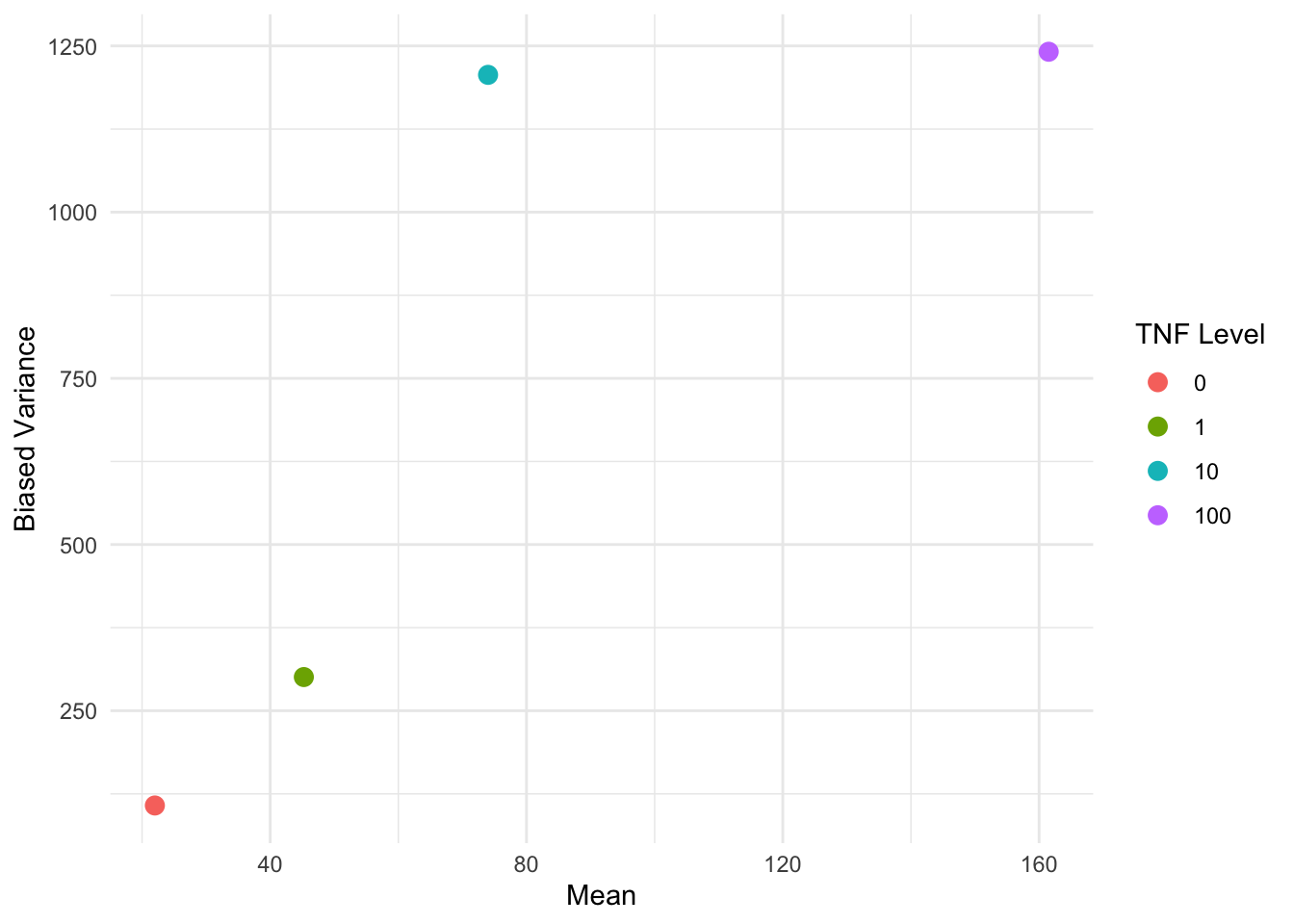

We can do a similar plot by IFN instead of TNF:

Code

variance_summary_by_IFN <- cells_tbl |>
    group_by(IFN) |>
    summarize(
        est_var = var(y) * 3 / 4,
        est_mean = mean(y),
        .groups = "drop"
    )
ggplot(variance_summary_by_IFN, aes(x = est_mean, y = est_var, color = factor(IFN))) +
    geom_point(size = 3) +
    labs(
        x = "Mean",
        y = "Biased Variance",
        color = "IFN Level"
    ) +
    theme_minimal()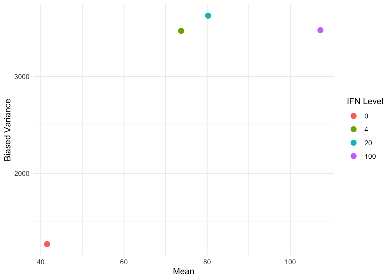

ggplot2 Syntax Explanation

ggplot(data, aes(...)): Initialize plot with aesthetic mappings (x, y, color, size, etc.)
- color = factor(TNF): Convert numeric to factor for discrete coloring
geom_point(): Add scatter plot layer
labs(): Set axis and legend labels (color = "TNF Level" customizes legend title)
theme_minimal(): Apply clean theme
Layers combined with + (similar to piping)

The equivalent base R code to create the same scatter plot would be:

Code

plot(
    variance_summary_by_TFN$est_mean,
    variance_summary_by_TFN$est_var,
    xlab = "Mean",
    ylab = "Biased Variance"
)

The non-linear relationship between the variance and the means suggests that we should consider some non-linear variance structures. In particular, we compare:

$\sigma^2(\mu) = \phi \mu$ (linear)
$\sigma^2(\mu) = \phi \mu^2$ (quadratic)
$\sigma^2(\mu) = \phi \mu + {\phi}_2 \mu^2$ (linear + quadratic—not explored here).

We leave the linear + quadratic case for further exploration.

Fit GEE with Linear Variance

We will now use the gee() function for “robust inference”. This means that we do not assume that the variance structure is correctly specified, but instead use the sandwich variance estimator for inference. We now try to partially replicate Table 2.7 from Fahrmeir and Tutz (2001), adapted below:

Log-linear model fits to cellular differentiation data based on quasi-likelihoods (Table 2.7, p. 60)
Parameter	$\sigma^2(\mu) = \phi\mu$	$\sigma^2(\mu) = \phi\mu^2$
`1`	3.436 (0.0)	3.394 (0.0)
`TNF`	0.016 (0.0)	0.016 (0.0)
`IFN`	0.009 (0.0)	0.009 (0.003)
`TNF*IFN`	-0.001 (0.22)	-0.001 (0.099)
$\hat{\phi}$	11.734	0.243

We start by considering the linear variance structure $\sigma^2(\mu) = \phi \mu$.

Code

gee_mu <- gee(
    formula = y ~ TNF * IFN,
    id = seq_len(nrow(cells_tbl)),
    data = cells_tbl,
    family = quasi(variance = "mu", link = "log")
)

Beginning Cgee S-function, @(#) geeformula.q 4.13 98/01/27

running glm to get initial regression estimate

  (Intercept)           TNF           IFN       TNF:IFN 
 3.435636e+00  1.552810e-02  8.946132e-03 -5.669994e-05

gee() Syntax Explanation

id: Cluster identifier for which observations are correlated. Here seq_len(nrow(cells_tbl)) creates unique IDs (1, 2, …, n) for each row, treating observations as independent
family = quasi(variance = "...", link = "..."): Specifies the assumed variance function and link function
- variance = "mu": Linear variance structure $\sigma^2(\mu) = \phi \mu$
- link = "log": Log link function

Code

gee_mu_summary <- summary(gee_mu)
gee_mu_summary


 GEE:  GENERALIZED LINEAR MODELS FOR DEPENDENT DATA
 gee S-function, version 4.13 modified 98/01/27 (1998) 

Model:
 Link:                      Logarithm 
 Variance to Mean Relation: Poisson 
 Correlation Structure:     Independent 

Call:
gee(formula = y ~ TNF * IFN, id = seq_len(nrow(cells_tbl)), data = cells_tbl, 
    family = quasi(variance = "mu", link = "log"))

Summary of Residuals:
      Min        1Q    Median        3Q       Max 
-44.70834 -14.92057  -6.49156  22.60660  44.16668 


Coefficients:
                 Estimate   Naive S.E.   Naive z  Robust S.E.  Robust z
(Intercept)  3.435636e+00 0.2184496319 15.727361 1.851532e-01 18.555643
TNF          1.552810e-02 0.0028462236  5.455686 2.329065e-03  6.667096
IFN          8.946132e-03 0.0033121255  2.701024 3.242937e-03  2.758652
TNF:IFN     -5.669994e-05 0.0000461918 -1.227489 3.598629e-05 -1.575599

Estimated Scale Parameter:  11.73516
Number of Iterations:  1

Working Correlation
     [,1]
[1,]    1

We can see now that the dispersion estimate is the same as the one we manually calculated based on Pearson residuals. We compare the coefficients and standard errors to the previous models:

Code

round(gee_mu_summary$coefficients, 4)

            Estimate Naive S.E. Naive z Robust S.E. Robust z
(Intercept)   3.4356     0.2184 15.7274      0.1852  18.5556
TNF           0.0155     0.0028  5.4557      0.0023   6.6671
IFN           0.0089     0.0033  2.7010      0.0032   2.7587
TNF:IFN      -0.0001     0.0000 -1.2275      0.0000  -1.5756

Code

round(glm_quasi_poisson_summary$coefficients, 4)

            Estimate Std. Error t value Pr(>|t|)
(Intercept)   3.4356     0.2184 15.7274   0.0000
TNF           0.0155     0.0028  5.4557   0.0001
IFN           0.0089     0.0033  2.7010   0.0193
TNF:IFN      -0.0001     0.0000 -1.2275   0.2432

The coefficients are be identical to the previous models, since the same score function is being solved. We can see that the naive standard errors are those assuming the variance structure is correct, while the robust standard errors are those using the sandwich variance estimator.

Why use the sandwich variance estimator? Expand for answer.

The sandwich variance estimator is “robust” because it is guaranteed to be asymptotically correct even if the variance structure is misspecified. If we incorrectly assume $\sigma^2(\mu) = \phi\mu$ when the true structure is different, the naive standard errors will be biased, but the sandwich estimator will still provide valid inference.

We can then calculate the $p$-values corresponding to the naive and robust standard errors.

Understanding the z-value Calculation

diag(...) extracts the diagonal elements from a matrix (variance-covariance matrix in this case). Standard errors are obtained by taking the square root of these diagonal elements: sqrt(diag(covariance_matrix)). Dividing the coefficient by its standard error gives the z-value.

Assuming we have correctly specified the variance structure (naive approach):

Code

naive_z_values <- tibble(
    coefficient = names(gee_mu$coefficients),
    z_value = gee_mu$coefficients / sqrt(diag((gee_mu)$naive.variance)),
    p_value = round(2 * pnorm(abs(z_value), lower.tail = FALSE), 3)
)
naive_z_values

# A tibble: 4 × 3
  coefficient z_value p_value
  <chr>         <dbl>   <dbl>
1 (Intercept)   15.7    0    
2 TNF            5.46   0    
3 IFN            2.70   0.007
4 TNF:IFN       -1.23   0.22

Without assuming the variance structure is correct (robust approach):

Code

robust_z_values <- tibble(
    coefficient = names(gee_mu$coefficients),
    z_value = gee_mu$coefficients / sqrt(diag((gee_mu)$robust.variance)),
    p_value = round(2 * pnorm(abs(z_value), lower.tail = FALSE), 3)
)
robust_z_values

# A tibble: 4 × 3
  coefficient z_value p_value
  <chr>         <dbl>   <dbl>
1 (Intercept)   18.6    0    
2 TNF            6.67   0    
3 IFN            2.76   0.006
4 TNF:IFN       -1.58   0.115

Warning

Note that in Fahrmeir and Tutz (2001) Table 2.7, the $p$-values of the $\sigma^2(\mu) = \phi \mu$ column corresponds to the naive $p$-values, whereas they should actually correspond to the robust $p$-values (read ahead below).

Expand the following note for an alternative implementation of GEE models using the geepack package.

Alternative geepack Implementation

There is an alternative package geepack which also implements GEE models. Under the hood, there are some small differences in implementation between gee and geepack.

Code

geepack_mu <- geeglm(
    formula = y ~ TNF * IFN,
    family = poisson(link = "log"),
    data = cells_tbl,
    id = seq_len(nrow(cells_tbl))
)
geepack_mu


Call:
geeglm(formula = y ~ TNF * IFN, family = poisson(link = "log"), 
    data = cells_tbl, id = seq_len(nrow(cells_tbl)))

Coefficients:
  (Intercept)           TNF           IFN       TNF:IFN 
 3.435636e+00  1.552810e-02  8.946132e-03 -5.669994e-05 

Degrees of Freedom: 16 Total (i.e. Null);  12 Residual

Scale Link:                   identity
Estimated Scale Parameters:  [1] 8.801367

Correlation:  Structure = independence  
Number of clusters:   16   Maximum cluster size: 1

Code

geepack_mu_summary <- summary(geepack_mu)
geepack_mu_summary


Call:
geeglm(formula = y ~ TNF * IFN, family = poisson(link = "log"), 
    data = cells_tbl, id = seq_len(nrow(cells_tbl)))

 Coefficients:
              Estimate    Std.err    Wald Pr(>|W|)    
(Intercept)  3.436e+00  1.852e-01 344.312  < 2e-16 ***
TNF          1.553e-02  2.329e-03  44.450 2.61e-11 ***
IFN          8.946e-03  3.243e-03   7.610   0.0058 ** 
TNF:IFN     -5.670e-05  3.599e-05   2.483   0.1151    
---
Signif. codes:  0 '***' 0.001 '**' 0.01 '*' 0.05 '.' 0.1 ' ' 1

Correlation structure = independence 
Estimated Scale Parameters:

            Estimate Std.err
(Intercept)    8.801   1.944
Number of clusters:   16  Maximum cluster size: 1

Fit GEE with Quadratic Variance

Finally, we try the quadratic variance structure $\sigma^2(\mu) = \phi \mu^2$.

Code

gee_mu2 <- gee(
    formula = y ~ TNF * IFN,
    id = seq_len(nrow(cells_tbl)),
    family = quasi(variance = "mu^2", link = "log"),
    data = cells_tbl
)

Beginning Cgee S-function, @(#) geeformula.q 4.13 98/01/27

running glm to get initial regression estimate

(Intercept)         TNF         IFN     TNF:IFN 
  3.393e+00   1.626e-02   9.433e-03  -6.011e-05

Code

gee_mu2_summary <- summary(gee_mu2)
gee_mu2_summary


 GEE:  GENERALIZED LINEAR MODELS FOR DEPENDENT DATA
 gee S-function, version 4.13 modified 98/01/27 (1998) 

Model:
 Link:                      Logarithm 
 Variance to Mean Relation: Gamma 
 Correlation Structure:     Independent 

Call:
gee(formula = y ~ TNF * IFN, id = seq_len(nrow(cells_tbl)), data = cells_tbl, 
    family = quasi(variance = "mu^2", link = "log"))

Summary of Residuals:
    Min      1Q  Median      3Q     Max 
-49.322 -16.653  -6.135  17.683  43.290 


Coefficients:
              Estimate Naive S.E. Naive z Robust S.E. Robust z
(Intercept)  3.393e+00  1.863e-01 18.2156   1.834e-01   18.499
TNF          1.626e-02  3.707e-03  4.3861   2.284e-03    7.118
IFN          9.433e-03  3.651e-03  2.5840   3.158e-03    2.987
TNF:IFN     -6.011e-05  7.265e-05 -0.8274   3.638e-05   -1.652

Estimated Scale Parameter:  0.2435
Number of Iterations:  1

Working Correlation
     [,1]
[1,]    1

Code

round(gee_mu2_summary$scale, 3)

[1] 0.244

The coefficients almost match those in Fahrmeir and Tutz (2001) Table 2.7 on page 60.

For a final sanity check, we manually compute both the naive and robust $Z$ and $p$-values.

Code

gee_mu2_inference <- tibble(
    coefficient = names(gee_mu2$coefficients),
    naive_z = gee_mu2$coefficients / sqrt(diag(gee_mu2$naive.variance)),
    naive_p = round(2 * pnorm(abs(naive_z), lower.tail = FALSE), 3),
    robust_z = gee_mu2$coefficients / sqrt(diag(gee_mu2$robust.variance)),
    robust_p = round(2 * pnorm(abs(robust_z), lower.tail = FALSE), 3)
)
gee_mu2_inference

# A tibble: 4 × 5
  coefficient naive_z naive_p robust_z robust_p
  <chr>         <dbl>   <dbl>    <dbl>    <dbl>
1 (Intercept)  18.2     0        18.5     0    
2 TNF           4.39    0         7.12    0    
3 IFN           2.58    0.01      2.99    0.003
4 TNF:IFN      -0.827   0.408    -1.65    0.099

Unlike for the linear variance structure, for the quadratic variance structure, the robust $p$-values match the ones in Fahrmeir and Tutz (2001). This confirms that all the $p$-values reported in parentheses of Table 2.7 of Fahrmeir and Tutz (2001) should have been robust $p$-values.

Code

packages <- c("conflicted", "dplyr", "Fahrmeir",  "gee", "geepack", "ggplot2", "MASS")
for (pkg in packages) {
    cit <- citation(pkg)

    # Check if multiple citations
    if (length(cit) > 1) {
        cat("- **", pkg, "**:\n", sep = "")
        for (i in seq_along(cit)) {
            cit_text <- format(cit[i], style = "text")
            cat("    - ", cit_text, "\n\n", sep = "")
        }
    } else {
        cit_text <- format(cit, style = "text")
        cat("- **", pkg, "**: ", cit_text, "\n\n", sep = "")
    }
}

conflicted: Wickham H (2023). conflicted: An Alternative Conflict Resolution Strategy. R package version 1.2.0, https://github.com/r-lib/conflicted, https://conflicted.r-lib.org/.
dplyr: Wickham H, François R, Henry L, Müller K, Vaughan D (2026). dplyr: A Grammar of Data Manipulation. R package version 1.2.0, https://github.com/tidyverse/dplyr, https://dplyr.tidyverse.org.
Fahrmeir: Halvorsen cbKB (2016). Fahrmeir: Data from the Book “Multivariate Statistical Modelling Based on Generalized Linear Models”, First Edition, by Ludwig Fahrmeir and Gerhard Tutz. R package version 2016.5.31.
gee: Carey VJ (2024). gee: Generalized Estimation Equation Solver. R package version 4.13-29.
geepack:
- Halekoh U, Højsgaard S, Yan J (2006). “The R Package geepack for Generalized Estimating Equations.” Journal of Statistical Software, 15/2, 1-11.
- Yan J, Fine JP (2004). “Estimating Equations for Association Structures.” Statistics in Medicine, 23, 859-880.
- Yan J (2002). “geepack: Yet Another Package for Generalized Estimating Equations.” R-News, 2/3, 12-14.
- Xu, Z., Fine, P. J, Song, W., Yan, J. (2025). “On GEE for mean-variance-correlation models: Variance estimation and model selection.” Statistics in Medicine, 44, 1-2.
ggplot2: Wickham H (2016). ggplot2: Elegant Graphics for Data Analysis. Springer-Verlag New York. ISBN 978-3-319-24277-4, https://ggplot2.tidyverse.org.
MASS: Venables WN, Ripley BD (2002). Modern Applied Statistics with S, Fourth edition. Springer, New York. ISBN 0-387-95457-0, https://www.stats.ox.ac.uk/pub/MASS4/.

References

Bartlett, Jonathan. 2014. “Deviance Goodness of Fit Test for Poisson Regression.” The Stats Geek. https://thestatsgeek.com/2014/04/26/deviance-goodness-of-fit-test-for-poisson-regression/.

Fahrmeir, Ludwig, and Gerhard Tutz. 2001. Multivariate Statistical Modelling Based on Generalized Linear Models. Second Edition. Springer Series in Statistics. New York, NY: Springer. https://doi.org/10.1007/978-1-4757-3454-6.

“Poisson Distribution.” 2026. Wikipedia. https://en.wikipedia.org/w/index.php?title=Poisson_distribution&oldid=1335765635.

Venables, W. N., and B. D. Ripley. 2002. Modern Applied Statistics with S. Fourth. New York: Springer. https://www.stats.ox.ac.uk/pub/MASS4/.